Statistics in Julia
I took a course on multivariate statistics and the instructor was very committed to the idea of demonstrating the quality of any claimed asymptotic results by running simulations. He did everything in R which I do not like and I took the opportunity to see what Julia was like for this kind of work.
The demonstration below looks at the test statistic for a comparison of multivariate normal sample means, if you have two groups and are not willing to assume that they have the same underlying covariance structure. In this case both the test statistic (Hotelling’s $T^2$) and one of the distribution parameters (the degrees of freedom $\nu$ in the $F$ distribution) depend on the observed data.
Start with imports, a convenient function for a random positive-definite matrix and a container of all the experimental architecture.
using Distributions, Parameters, Statistics, Random
using LinearAlgebra, Plots, LaTeXStrings, ProgressMeter
Random.seed!(420);

"Generate random positive definite matrix of given dimension."
function Σ(p)
    m = qr(reshape(rand(Normal(), p^2), (p, p))).Q
    Hermitian(m' * (m .* reverse(collect(1:p))))
end;

"Struct of parameters which define the experiment architecture."
@with_kw struct Params
    # Sample dimensions.
    p = 3; nx = 8; ny = 12
    # True means and variances.
    μx = [4, 3, 2]; μy = [4.1, pi, 1.9]
    Σx = Σ(p); Σy = Σ(p)
end;
Then calculate the test statistic and degrees of freedom given observed data. The math is a bit involved but that’s not the main thing here.
function Hotelling(x, y, Sx, Sy, nx, ny)
    xbar = mean(x, dims=1)'; ybar = mean(y, dims=1)'
    ((xbar - ybar)' * inv(Sx/nx + Sy/ny) * (xbar - ybar))[1]
    end;

function ν(Sx, Sy, nx, ny)
    p = size(Sx)[1]
    a(S, n) =  1/n * S * inv(Sx/nx + Sy/ny)
    ax = a(Sx, nx); ay = a(Sy, ny)
    b(a) = tr(a^2) + tr(a)^2
    (p + p^2) / (1 / nx * b(ax) + 1 / ny * b(ay))
    end;
This is the main function, which draws two random samples in line with the given configuration parameter and then returns the test statistic and degrees of freedom. This will be run many times.
"Run one trial, that is generate an F statistic and ν  from the experimental design in P.
The claim is that T2 is distributed as νp/(ν - p + 1)F(p, ν - p + 1)."
function trial(P::Params)
    x = rand(MvNormal(P.μx, P.Σx), P.nx)'
    y = rand(MvNormal(P.μy, P.Σy), P.ny)'
    Sx = cov(x); Sy = cov(y)
    T2 = Hotelling(x, y, Sx, Sy, P.nx, P.ny)
    nu = ν(Sx, Sy, P.nx, P.ny)
    F = (nu - P.p + 1) / (nu * P.p) * T2
    [F, nu]
    end;
We just collect the outputs from many calls of the trial function above and plot them.
Some of the Julia code feels clunky since I’m fairly new to this language.
P = Params();
data = @showprogress [trial(P) for _ in 1:10^6]
f = [first(x) for x in data];
nu = [last(x) for x in data];
histogram2d(nu, f, title="F vs. ν", xlabel="ν", ylabel="F", ylims=(0, 25))
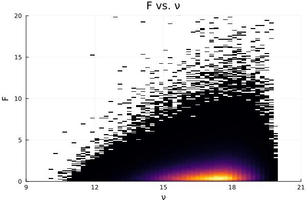
2d Histogram of $T^2$ and $\nu$.
We can take a few vertical slices from the plot above and compare them to the approximating distribution:
function vis(νbar, legend=false)
    histogram(
        f[νbar - .5 .< nu .< νbar + 5],
        normalize=:true,
        label="Empirical",
        xlims=(0, 4),
        title=L"$\nu =$" * "$νbar",
        legend_position=legend)
    d = FDist(P.p, νbar - P.p + 1);
    plot!(x -> pdf.(d, x), lw=3, label="Approximate")
    end
p = plot(vis(10), vis(14, true), vis(18),
plot_title="Approximate Distribution of Hotelling's " * L"T^2",
layout=(3, 1),
size=(900, 600))
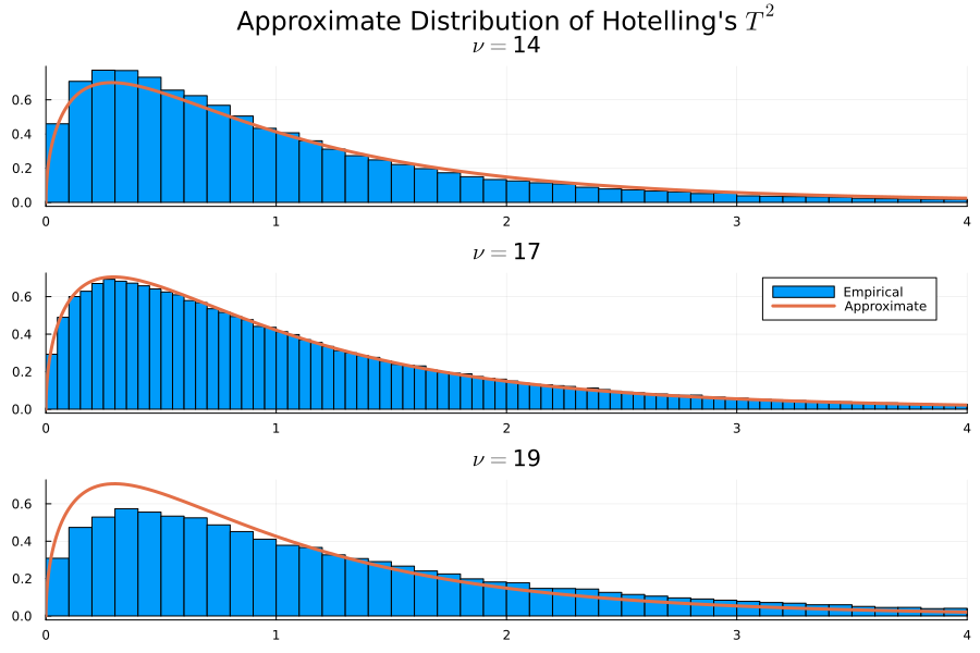
True vs. approximate distribution of test statistic.